Matlab For Engineering

• I used Matlab to solve basic analytical engineering problems as part of my 1st year mechanics module.

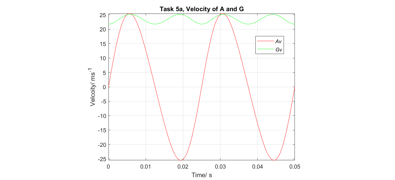
I used basic calculus to calculate and plot linear velocity data from a piston of given geometry over 2 rotations.

[AB,BC,BG,W,t]=deal(0.6,0.1,0.08,(40*2*pi),sym('t'));%define dimensions and algebraic variables.
theta=W*t; %define angle in terms of angular speed and time
tlim = 2/40; %define time for 2 cycles
alpha=asin((BC/AB)*sin(theta));%define geometry of problem
AC = -AB*(cos(alpha)) -(BC*cos(theta));%expression for displacement AC
Av=diff(AC)

GAvector=[-BC*cos(theta)-BG*cos(alpha),(BC*sin(theta)-BG*sin(alpha))]; %vector containing i and j components of displacement AG
Gvvector=diff(GAvector); %differentiate displacement vector 
Gv=norm(Gvvector)%find the magnitude of the veloicty vector
fplot(Gv,[0 tlim],'g'); %plot velocity of G within time intervals

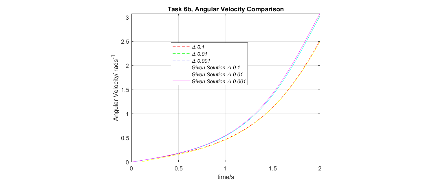
I used iterative methods with different time steps to plot a ladder sliding down a wall before comparing it to a closed form solution

for i=(1:N3); %count i from 1 to number of steps (0.001 for third for loop)
  t3(i+1)=t3(i)+h3;
  theta3(i+1)=theta3(i)+h3*(omega3(i));
  alpha3(i)=(3*g*sin(theta3(i))/8);
  omega3(i+1)=omega3(i)+h3*(alpha3(i));
end
plot(t3,theta3,'b'); %plot angular position against time for 0.001
      

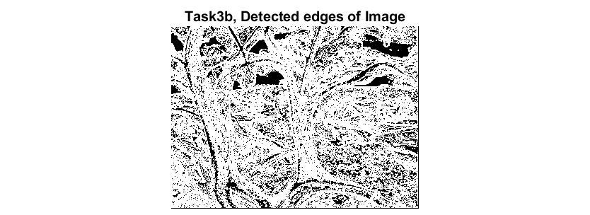
Edge Detection Applied to Matlab Trees Picture

I implemented a basic edge detection function that could be applied to different images with a variable threshold.

function output = edge_detection(input);%define sub function 
  I = imread(input); %read the input
  [Iwidth,Iheight] = size(I); %define size of I
  C = zeros(size(I)); %create an array of zeros 
  for i = 1:(Iwidth-1); %count along the rows to the penultimate value
      for j = 1:(Iheight-1);%count down the columns to the penultimate value
          if I(i,j) + threshold => I(i+1,j); %If adjacent pixels are different return 1
             C(i,j)=1;
          elseif I(i,j) ~= I(i,j+1);%if adjacent pixels are the same return 0
             C(i,j)=1;
          end
       end
   end