Matlab Robotic Arm

Robotics

Matlab

Software

I used Matlab to construct a kinematic model of a 3D robotic arm using the DH convention. I tested, analysed and visualised the model.

Plotting the robot's trajectory in joint space and cartesian space.

I assigned reference frames to each link of the robots arm using the Denavit-Hartenberg convention.

% create a DH table: ai alphai di thetai
  DH = [0         0       0.2703  theta1;...  %Joint 1
        0.069     -pi/2   0       theta2;...  %Joint 2
        0         pi/2    0.3644  theta3;...  %Joint 3
        0.069     -pi/2   0       theta4;...  %Joint 4
        0         pi/2    0.3743  theta5;...  %Joint 5
        0.01      -pi/2   0       theta6;...  %Joint 6
        0         pi/2    0.2295  theta7];    %Joint 7

I constructed a transformation matrix from the base of the robot to the end-effector.

for i = 1:TN
T(i).A =  [cos(theta(i)) -sin(theta(i)) 0 a(i);...
    sin(theta(i))*cos(alpha(i)) cos(theta(i))*cos(alpha(i)) -sin(alpha(i)) -sin(alpha(i))*d(i);...
    sin(theta(i))*sin(alpha(i)) cos(theta(i))*sin(alpha(i)) cos(alpha(i)) cos(alpha(i))*d(i);...
    0 0 0 1];
end

Visualisation of the kinematic model

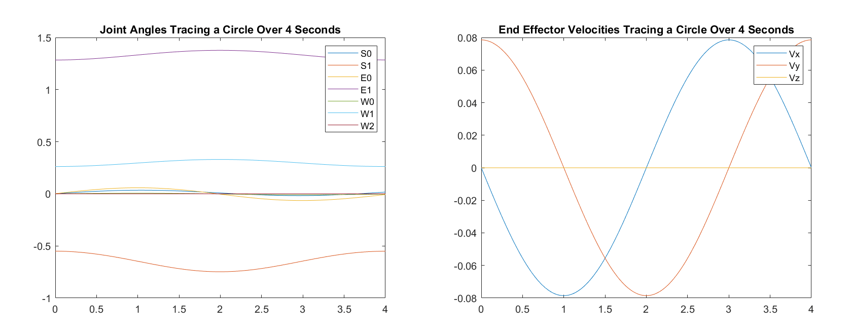
I wrote a script that could take a cartesian function as an input and calcualte the joint angles at set time increments.

for t = 0:dt:4
  NewJacobianMatrix = vpa(subs(JacobianMatrix,[theta1,theta2,theta3,theta4,theta5,theta6,theta7],transpose(newjointangles))); %substitute angles into Jacobian matrix
  newjointangles = simplify(newjointangles + dt*(pinv(NewJacobianMatrix)*[-(pi*sin((pi*t)/2))/40; (pi*cos((pi*t)/2))/40; 0])); % multiply cartesian function by the pseudo inverse of the Jacobian Matrix
  JointangleMatrix(:,j) = newjointangles; %append each set of joint angles to a larger matrix
  Endeffectorvel(:,j) = (NewJacobianMatrix * (pinv(NewJacobianMatrix)*[-(pi*sin((pi*t)/2))/40; (pi*cos((pi*t)/2))/40; 0]));%[-(pi*sin((pi*t)/2))/40 (pi*cos((pi*t)/2))/40 0]; %append the velocity of the end effector to a matrix
  pseudoinverseJacobianMatrix(:,:,j)= pinv(NewJacobianMatrix); %append each pseudo inverted jacobian matrix to a larger matrix
  JacobianMatrixMatrix(:,:,j)= NewJacobianMatrix; %append each jacobian matrix to a larger matrix
  Cartesianposition = Cartesianposition + dt*(NewJacobianMatrix * (pinv(NewJacobianMatrix)*[-(pi*sin((pi*t)/2))/40; (pi*cos((pi*t)/2))/40; 0]));
  Cartesianpositionmatrix(:,j) = Cartesianposition; %append the cartesian positions to a larger matrix
  j=j+1; %increase index variable
end

After the kinematic model was working I began experimenting with trajectories outside of the robot's workspace and poses that resulted in a singularity, effectively breaking the kinematic model.

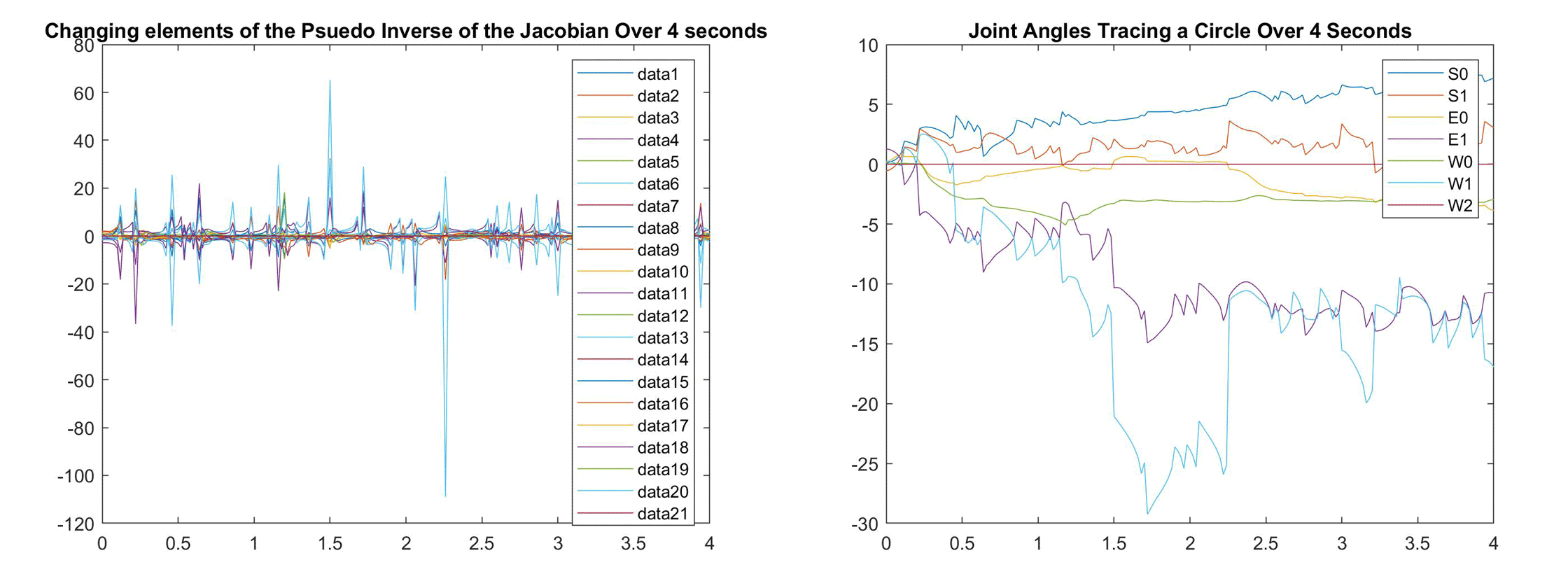
Plotting the pseudo-inverse of the jacobian and the joint angles for a "broken" trajectory

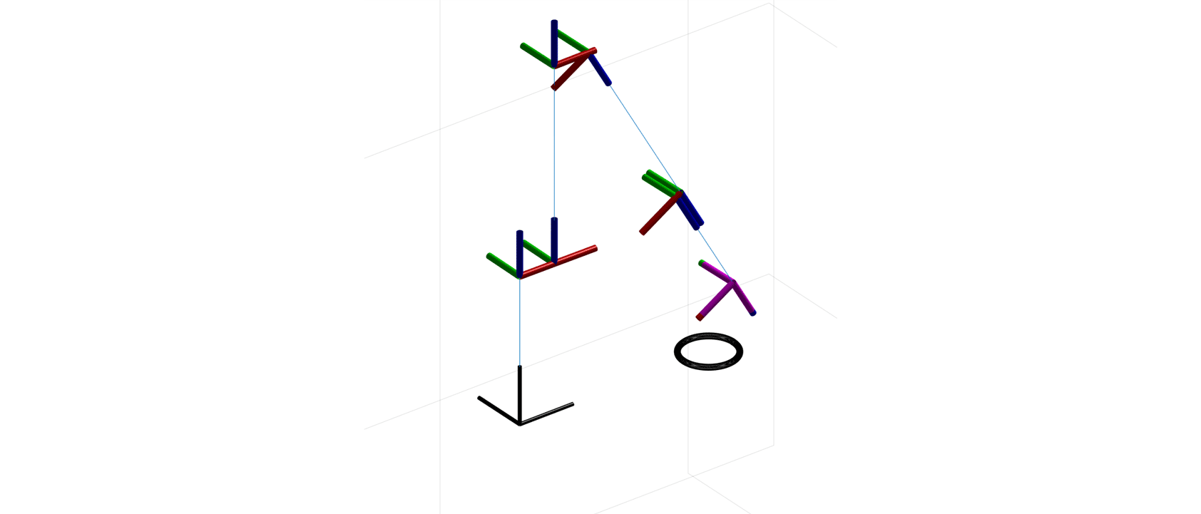
Visualisation

Finally I used the Matlab robotics toolbox to visualise my model in 3D by defining joints, reference frames and angular range.

Oli Thompson